Attention Diagnostics: Testing KL and Susceptibility on the IOI Circuit

Post 1 derived two per-head diagnostics from the structure of the softmax operator: KL selectivity \(\hat\rho_{\text{eff}} = \text{KL}(\hat\pi \| u)\) measures how sharply a head focuses its attention, and susceptibility \(\chi = \text{Var}_{\hat\pi}(\log\hat\pi)/(\log n)^2\) measures how sensitive that sharpness is to small changes in the query-key scores. Both are computed from a single forward pass — no gradients, no activation patching.

Here I test a concrete prediction: circuit heads should show larger shifts in these diagnostics between activating and non-activating prompts than non-circuit heads. The testbed is GPT-2-small’s Indirect Object Identification (IOI) circuit,¹ whose 23 heads and functional roles are well characterized.

Jupyter notebook with analysis here.

---

Recap

A prompt is a token sequence \(x = (x_1, \ldots, x_n)\). GPT-2-small processes it layer by layer, maintaining a residual stream \(h_i^{(l)} \in \mathbb{R}^{d_{\textrm{model}}}\) for each position — a contextualized representation that accumulates the contributions of all attention heads and MLPs up to layer \(l\).

Each of the 144 heads (12 layers × 12 heads) projects the residual stream into queries and keys, computes scores \(z_{ij} = q_i \cdot k_j / \sqrt{d_k}\), and applies softmax to produce an attention distribution over source positions:

\[\hat{\pi}_j = \text{softmax}(z_j).\]

This \(\hat{\pi}\) depends on both \(x\) (through the queries and keys) and the head’s learned parameters. From it we read off the two diagnostics introduced in Post 1:

\[\hat{\rho}_{\textrm{eff}} = {\text{KL}(\hat{\pi} \| u)}, \qquad \chi = \frac{\text{Var}_{\hat{\pi}}(\log \hat{\pi})}{(\log n)^2}, \label{eq:diagnostics}\]

where \(u = (1/n, \ldots, 1/n)\) is the uniform distribution. Note: Post 1 used the notation \(\partial\hat{\rho}\) for the temperature susceptibility; here we write \(\chi = \partial\hat{\rho}/(\log n)^2\). No backward pass needed — \(\hat{\pi}\) is already computed in the forward pass.

---

Experimental setup

GPT-2 small is known to have a circuit that performs indirect object identification.¹ Let’s say we have a prompt of 15 tokens that reads:

\[x = \textrm{When Alice and Bob went to the store,} \textbf{ Bob } \textrm{gave a drink to ___}. \label{eq:good_prompt}\]

The correct next token the model should predict is Alice (the indirect object of the second clause). It turns out that Wang et al. showed that several heads perform various jobs in order to predict this next token correctly. One head detects a name has appeared twice, another suppresses the name that has appeared twice, another moves the name that appeared once, and so forth.

For our experiments, we shall generate 50 IOI prompts of length \(n=15\) of exactly the same format as \eqref{eq:good_prompt} along with 50 non-IOI prompts that have a similar format but no repeating name, e.g.

\[x = \textrm{After Mary and John sat down for dinner,} \textbf{ Sarah } \textrm{gave a gift to ___}\]

which should not “activate” the circuit, and this should be reflected in a shift in the values of our diagnostics, \eqref{eq:diagnostics}.

All experiment details, code, and plots can be found in this notebook.

---

A single circuit head

Layer 9, head 9 (L9H9) is a Name Mover attention head, responsible for copying the correct indirect object name to the output. Below we see a noticeable difference between IOI and non-IOI prompts in the \((\rho, \chi)\)-plane (dropping the \(\hat{\quad}\) symbol and \(\textrm{eff}\) subscript for ease of notation).

Figure 1. L9H9 (Name Mover) in the \((\rho,\,\chi)\) plane. Red: IOI prompts (circuit active). Gray: non-IOI prompts (circuit inactive). Stars mark condition means.

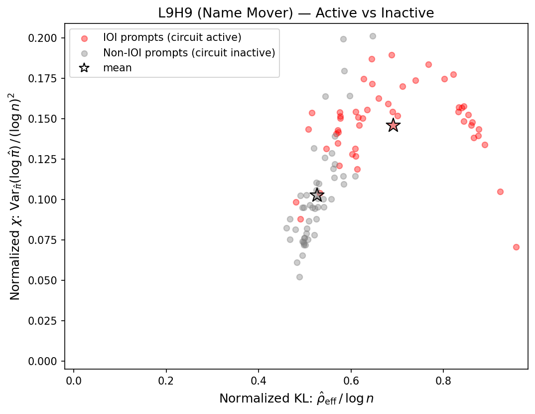
It looks like the diagnostics can show the difference between the head activating versus not!

It also seems like our hypothesis was correct: activating the circuit shifts the head toward higher KL selectivity, consistent with the prediction from Post 1.

Let’s check all 23 circuit heads.

---

All 23 circuit heads

Figure 2. All 23 IOI circuit heads organized by role. Each panel shows per-prompt \((\rho,\,\chi)\) for IOI (colored) and non-IOI (gray). Arrow: non-IOI mean → IOI mean.

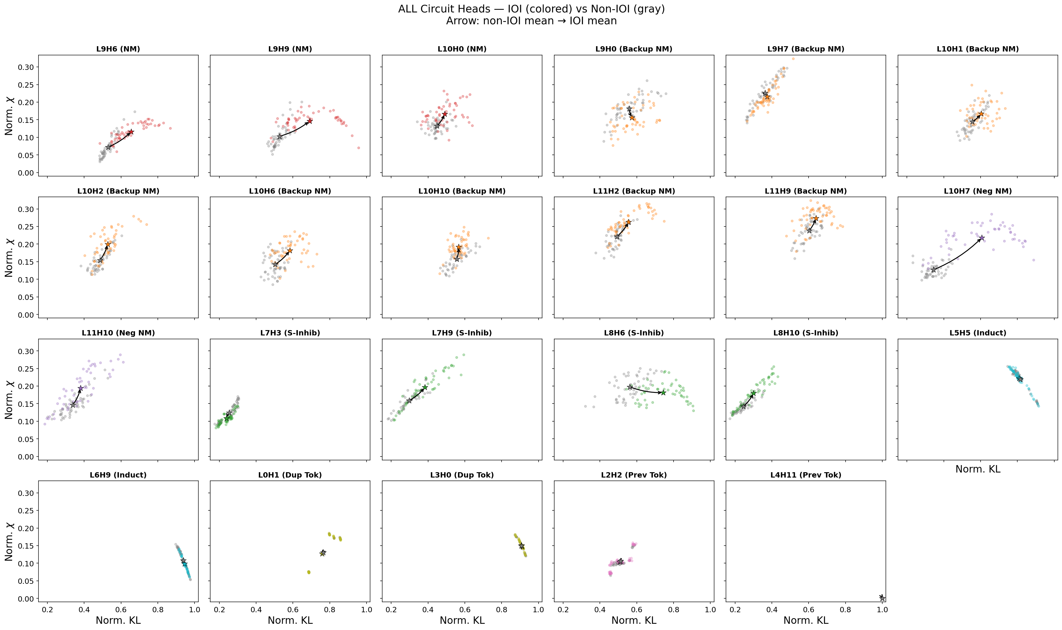
It seems that non-active-to-active experiments produce signal in our diagnostics, but such signal is role dependent. Name movers, backup name movers, negative name movers, and S-inhibition all show clear shifts; these heads only activate when the repeated name pattern appears. Induction, duplicate token, and previous token exhibit no shift; these are structural heads, which merely track patterns and positions among tokens, building up representations in earlier layers that the selection heads later consume. Their jobs do not change between prompt types.

It seems that some, though not all, circuit types share similar fingerprints in the \((\rho, \chi)\)-plane, suggesting an interesting future direction of research: can candidate circuit heads be identified via these fingerprints?

---

Non-circuit heads

For comparison, we can see that non-circuit heads tend to not show a shift in (\(\rho,\chi\)). For the quantity defined as

\[\Delta \mathrm{KL} = \langle \rho \rangle_{\textrm{IOI prompts}} - \langle \rho \rangle_{\textrm{non-IOI prompts}} \label{eq:delta_kl}\]

we show below those non-circuit heads with either one of top four values in \(|\Delta \mathrm{KL}|\) or the bottom twelve. Note that a few non-circuit heads do seem to activate on IOI prompts. Their precise role is unclear, but their attention patterns appear sensitive to syntactic features these prompts share — not to the IOI computation specifically.

Figure 3. Selected non-circuit heads. Orange: top-4 by |\(\Delta \) KL|. Blue: 12 inert heads with near-zero shift. Most non-circuit heads are indifferent to whether the IOI circuit fires.

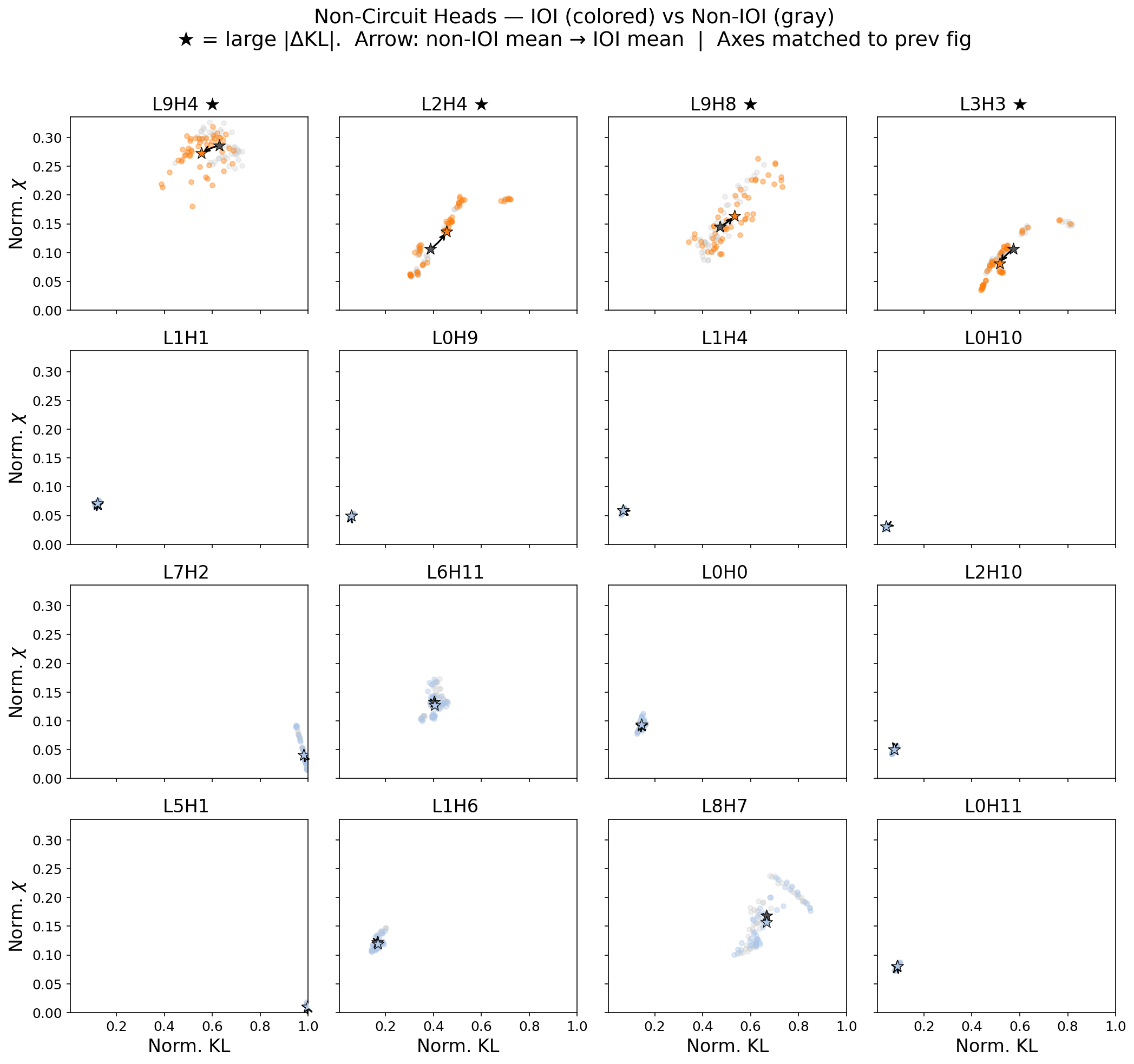
The existence of these outlier non-circuit heads means the separation is not perfect — but does it hold statistically, across all 144 heads?

---

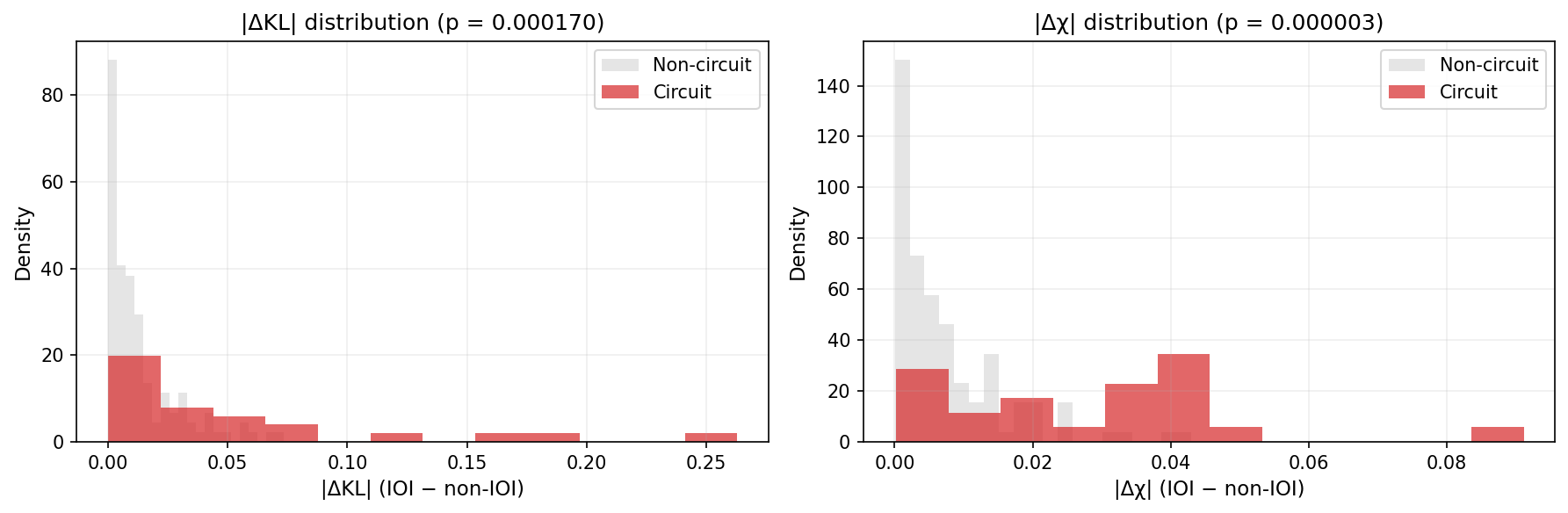
Statistical test: do the diagnostics separate circuit from non-circuit?

So can the shift from non-IOI to IOI prompts in the (\(\rho,\chi\)) plane distinguish between circuit and non-circuit heads? To test this hypothesis we rank the mean shifts in KL (\(\rho\)), as measured by Eq. \eqref{eq:delta_kl}, for each head. (And similarly for the mean shift in \(\chi\)). Does this ordering generically rank any given circuit head higher than a non-circuit head (that is, more often than it would do to chance for random orderings)?

This corresponds to the Mann-Whitney statistical test. We can see in our plots below that it is indeed statistically significant! Our p-values are \(p=0.0002\) and \(p<0.0001\) for the \(\Delta \mathrm{KL}\) and the \(\Delta \chi\) shifts, respectively.

Figure 4. Distributions of \(|\Delta\text{KL}|\) (left) and \(|\Delta\chi|\) (right) for circuit (red) vs non-circuit (gray) heads. Mann-Whitney U: \(p=0.00020\) and \(p<0.0001\) respectively.

---

Cross-head correlations: a teaser

The diagnostics so far treat heads independently. But heads in the same functional role don’t just shift in isolation — they tend to move together. Computing the 144×144 Pearson correlation matrix of KL selectivity across prompts reveals structure aligned with the circuit.

Figure 5. Cross-head KL correlation matrices. \(C_\text{IOI}\) and \(C_\text{non-IOI}\) are 144×144 Pearson correlation matrices computed across 50 prompts each; \(C_\text{diff} = C_\text{IOI} - C_\text{non-IOI}\) isolates task-specific coupling. Brown margin ticks mark the 23 known circuit heads.

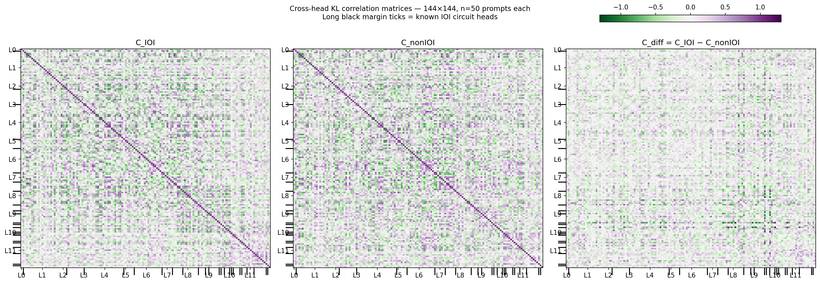
The idea is that \(C_\text{IOI}\) includes correlations both due to circuit activation and other typical interactions among heads for non-circuit behaviors. By subtracting off \(C_\text{non-IOI}\) we are subtracting the “baseline” non-circuit correlations, thereby isolating the circuit correlation structure in \(C_\text{diff}\). The above figure shows a promising sparsification in the correlation structure in \(C_\text{diff}\)—another promising future direction for possible circuit discovery.

Below we plot a scatter plot of every \((C_\text{IOI},\, C_\text{non-IOI})\) for all non-circuit (NC) to circuit head pairs (blue) and all NC to NC pairs. \(C_\text{diff}\) is the direction from the unity line.

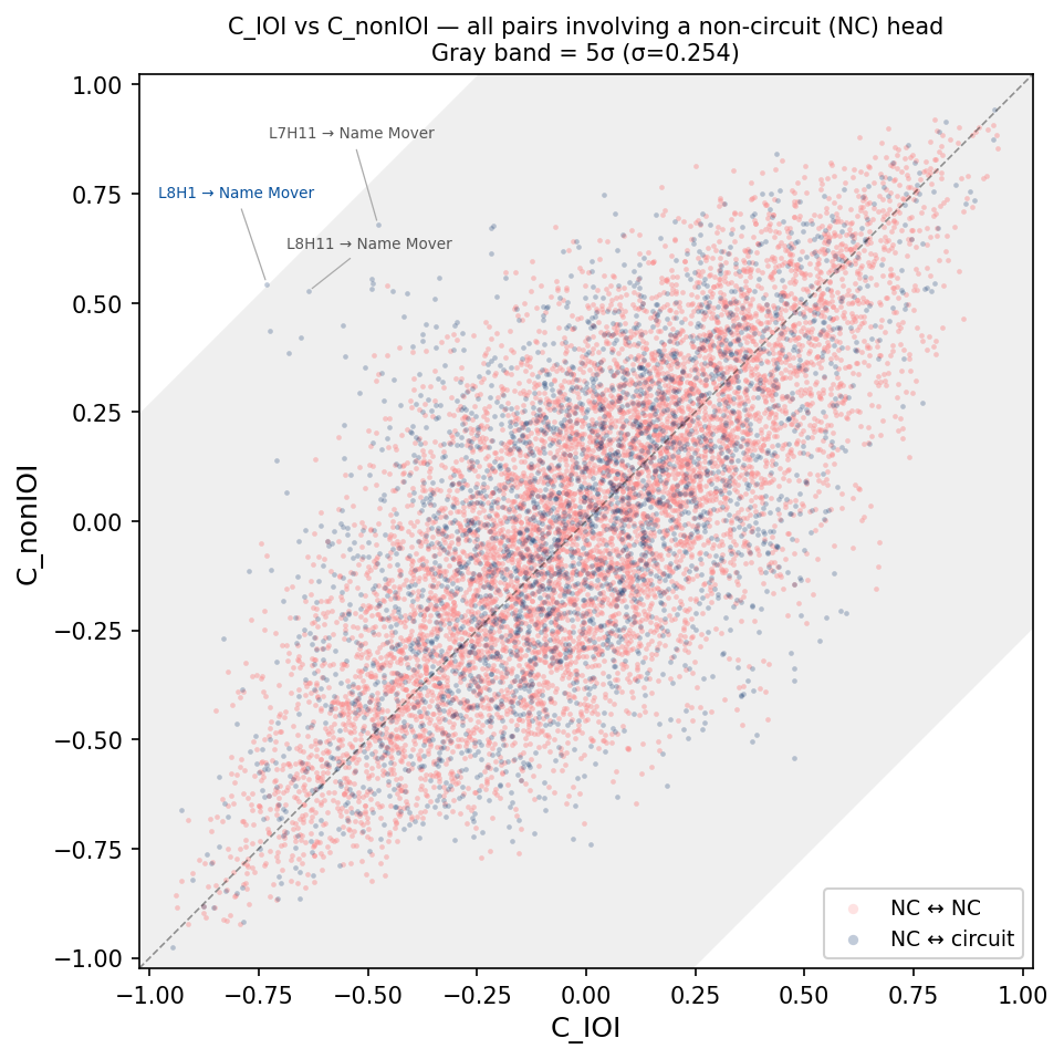
Figure 6. Every (NC head, other head) pair plotted as \((C_\text{IOI},\, C_\text{non-IOI})\). Points on the diagonal have \(C_\text{diff}=0\). The gray band is \(\pm 5\sigma\) of the empirical \(C_\text{diff}\) distribution. Blue: NC head paired with a circuit head; red: two NC heads. Labeled: the three NC heads with the largest \(

C_\text{diff}

\) coupling to a circuit head.

There is one attention head in layer 8 (L8H1) that shows a dramatic shift in its correlation to a name-mover head when the circuit is activated. In fact, it’s 5 standard deviations away from mean no-shift behavior (\(C_\text{diff}=0\)). Could it be another circuit head missed by the analysis in Wang et al.? Five standard deviations is good enough for declaring the discovery of a new particle in high energy physics, so it seems good enough for me!

(Just kidding). In all seriousness, it would be worth checking for any mechanistic relation between this and other high \(C_\text{diff}\) heads via typical ablation/patching techniques.

---

Limitations, implications, and next steps

Our diagnostic only observes behavior of the whole attention head for different prompts; it does not reveal mechanism for underlying computation on any kind of per-prompt basis. Additionally we expect attention to be more and more selective (higher KL) as we go into deeper layers, regardless of whether the head is inside the circuit or not. This confound needs to be accounted for. Nevertheless, the idea of similar fingerprints in the (\(\rho,\chi\))-plane for similar circuit elements along with the correlation analysis idea each show promise for unsupervised circuit discovery.

Natural next steps include validation of our diagnostics for other known circuits… we have in fact only tested out one circuit on one data set after all. Though seeing if L8H1 is in fact a circuit element initially missed by Wang et al. would be interesting in and of itself.

Furthermore, our correlation analysis does not account well for strong signal due to transitive correlation, i.e. circuit A and B show strong correlation not due to any inherent coupling, but due to mutual correlation to a third element C. In biological analyses of neurons and amino-acid sequences this is typically dealt with via Direct Coupling Analysis. DCA fits a maximum entropy model to a correlation matrix, and has shown meaningful success in uncovering real, underlying interactions among neurons/amino acids. Since we are showing different prompts to our LLM and tracking the responses for stable structure, this is very similar to analysis done by Hoshal and Holmes et al. in their neuro-theory article, “Stimulus-invariant aspects of the retinal code drive discriminability of natural scenes.”²

If our analysis can take correlation graphs and turn them into candidate circuit graphs, this would help narrow down to a few candidate heads for a given circuit computation. If so, this could be a promising direction for scaling up (and speeding up) circuit discovery methods, e.g. correlation analysis to find candidates followed by causal interventions to determine mechanism.

The significant \(\Delta\chi\) is also perhaps surprising — Post 1 predicted \(\chi\) should be low in both conditions, so we’d expect \(\Delta\chi \approx 0\). We’ll have to think a little bit more in a future post about what \(\chi\) is (or is not) actually capturing. (We note that Kim (2026)³ applies a related fluctuation-dissipation susceptibility to GPT-2 training dynamics, using it to detect grokking as a phase transition — a complementary direction to the inference-time head characterization pursued here.)

---

1. Wang et al. (2022). Interpretability in the Wild: a Circuit for Indirect Object Identification in GPT-2 small. ↩ ↩²

2. Hoshal et al. (2024). Stimulus-invariant aspects of the retinal code drive discriminability of natural scenes. PNAS 121(52):e2313676121. ↩

3. Kim, J. (2026). “Thermodynamic Isomorphism of Transformers,” arXiv:2602.08216. ↩